Connecting Google Colab compute instances to your data
It’s pretty indisputable that machine learning is both trendy and effective in a number of Earth & environmental sciences. With the speed and uptake of, particularly, deep-learning methods it’s hard to keep up with best practices for training and deploying models. It’s also expensive to roll your own hardware to build a DL platform for these applications, where data sizes can be large, heterogeneous, and generally difficult to wrangle. That is to say, the data space of Earth science is moving as fast as machine-learning. In well funded projects this isn’t necessarily a problem, but for exploring hypotheses and proofs-of-concept it’s important to have access to hardware that can be useful on limited timelines. Particularly, this can be a daunting landscape for students who are expected to learn the science and technology concurrently.
Okay, passive voice aside, this is a tough space to operate in. GPUs are absurdly expensive at the moment. Traditional HPC architectures don’t include GPUs. If you’re a student or working on an unfunded project you’re most likely working on either your laptop or an underpowered lab machine. Google Colab provides free (as in beer, not speech) access to some pretty good GPU and TPU resources that are most likely better than your laptop. The problem is you need to have data “local” to those instances to use them for free. For the most part, this is either through example datasets or by uploading your data to Google drive. Not exactly the best dichotomy. Either get slow compute by keeping all of your storage local or get slow/insufficient storage by having to upload huge datasets every time you make a tiny change to the preprocessing of your data. This post is about connecting your storage to Google’s compute in a way that scales pretty well for smaller (~10s of GB of data) but not “small” projects.
A minor warning
The example I’m going to give here considers drought prediction. I’m glossing over a ton in this space, and you best not try to use ML to predict extremes without much more careful thought on both your input data, data selection strategy, training approach, and model architecture.
The conceptual diagram
Before getting into details and code, I want to take a second to go over all the pieces that this post constructs. This conceptual diagram is shown below, in figure 1. The high level architecture here shows that there are two machines, one for storage and data manipulation as well as one for managing compute at training time.
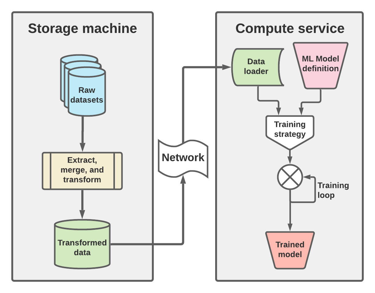
On the storage side (left portion of figure 1) the raw datasets are loaded, subsetted, transformed, and saved out into the intermediate format that will be used to train the machine learning model. Ideally this involves transformation into a data structure and file format that supports chunking and must be able to be loaded over network interfaces. In this post I will focus on using zarr, which not only supports both but is almost perfectly designed for such a workflow. The need for network access should be obvious here, given that the network is the mediator between the storage machine and compute service, but the need for “chunking” may not. To get a sense of how chunking can affect data latency, you can look back at my previous post on chunking NetCDF data. Though similar, in that post I was interested in optimizing writing output, while in this one I am more interested in reading input. In both cases, having a good chunking strategy is key, and further the chunking strategy we use here will be crucial to how we do mini-batch training on the compute service.
This manifests itself on the right hand side of figure 1, in the “Data loader” which is responsible for loading these minibatches, which will be consumed by the training strategy. Along with an ML model definition, this training strategy is iterated to optimize the best model, given the training data provided by the data loader. The output of this workflow is the trained model which then can be used in forward mode for whatever purpose it was designed for.
Step 1: The storage side (Here, zarr)
For all of the dataset manipulations I’ll assume use of xarray, since it’s
mostly become the standard way to access Eath science data for computationally
intensive studies. Assuming we have a number of datasets we load them up like
so
    import xarray as xr
    mod_ds = xr.open_dataset('/path/to/model_output.nc')
    ref_ds = xr.open_dataset('/path/to/reference.nc')
Now suppose we want to run a classification task where we have “reference
categories”
such as those derived by the US drought
monitor
that we want to train our ML model to predict. Given those have previously been
one hot
encoded
we similarly need a strategy to map our data from model_output.nc to such
encodings. We may also need to trim these modeled outputs to where we have
target/observed/truth data. These steps are what I will call the “Extract,
merge, transform” steps, which map well to the first two steps of the standard
extract, transform, load (ETL) workflow pattern.
For the sake of the post, let’s assume we have gridded drought indicators which
span from \(W^4\)-\(W^0\) (for wet-period–4 through 0), \(N\) (for neutral),
and
\(D^0-D^4\) (for drought-period-0 through 4) which have been encoded into 11
categories in our reference.nc dataset(s).
If we assume (and this is a big assumption) that we can map the modeled quantiles of soil moisture (SM) and snow water equivalent (SWE) to these categories in some fashion we would like to transform these modeled outputs to data that is amenable to learning such a mapping. Like most machine learning this requires transforming data to be closer to normal and roughly on a scale of \(\pm 1\). Luckily for us quantiles are inherently in the range of 0-1, though probably in a very skewed distribution. Glossing over the skewedness (which you most certainly do need to deal with in real life)…
In psuedo-code, this looks like:
    quantiles_of = xr.Dataset()
    var_list = ['soil_moisture', 'snow_water_equivalent']
    for var in var_list:
        quantiles_of[var] = quantiles(var)  # code excluded for brevity
Given our initial simulation data we might get some data which has quantiles
with dimensions (time, lat, lon) or some similar arangement. From this let’s
assume we want our ML model to see some maximum time period for each grid cell
(that is, time dependence but no spatial dependence). This is another very
strong assumption, but considerably simplifies this post. In doing this we need
to generate samples which have dimensions (time_lookback, number_features)
where time_lookback is a hyperparameter and number_features is 2 wheare
feature 0 is soil moisture and feature 1 is snow_water_equivalent.
To accomplish this you might imagine more pseudo-code:
    samples_list = []
    space_list = ['lat', 'lon']
    z_ds = quantiles_of.stack(z=space_list)
    for i in range(z_ds['z']):
        samples_list.append(make_lookback(z_ds.isel(z=i), time_lookback=180))
    lookback_ds = xr.concat(samples_list, dim='samples')
This gives a new dataset with dimensions (samples, time_lookback, features),
which is compatible with something like the Keras LSTM
layer or PyTorch LSTM
layer (provided
batch_first is set to True). With this, it’s time to set up chunking along
the sample dimension to exceed what we will use as the batch size on the
compute
side. Knowing what to set this as depends a bit on the size of lookback and the
number of features, as well as the available memory on the compute side, but
generally you want this to be as large as possible to fit in memory on the
other
side. Here I’ll just assume a chunk size of 10,000 for no particular reason.
Then
we’ll save out the dateset to a zarr
store.
This is easily accomplished just by doing:
    lookback_ds = lookback_ds.chunk({'samples': 10000})
    lookback_ds.to_zarr(OUTPUT_PATH, consolidated=True)
Now, the only thing of note here is that OUTPUT_PATH should be readable over
the network (aka this directory should be served up over something like HTTP or
FTP).
Step 2: The network interface (Here, fsspec)
So now we enter the middle part of figure 1, where we need to
be able to transfer the data from the storage system to the compute system in
an automated, and robust way. To do so we’ll leverage the excellent fsspec
library. There actually
isn’t
anything to do here, except make sure that your data is accessible via the web
and that you can install fsspec on the compute server. I suppose it’s worth
pointing out here that you probably want to host your data on a fast network.
As this post is targeted at folks who work at Universities or similar
institutions,
you probably want to host this on their networks since they’ll most likely be
much faster than your own home network. There are tons of resources out there
on this topic that are going to be much better than anything that I could write
up so I’ll leave this one up to you! With that laid out, let’s move on to how
you actually acccess this data on the other side.
Step 3: The compute service (Here, Google colab)
On the right hand side of figure 1 we need three main things:
- A data loader that can access the data we created in step 1 over the network in an efficient way.
- A machine-learning model definition
- A Training strategy to optimize the model given the data
Generally, the last two are outside of the scope of this post, but I’ll give
examples for the sake of completeness. The first component however, bears some
explanation. But before we get to how to process the data for ingesting into
our machine learning model we should discuss a bit of infrastructure which is
specific to Google Colab. I’m not going to get too deep into how to use Colab
or it’s features but you can learn more here:
https://colab.research.google.com/?utm_source=scs-index. Generally Colab
provides an easy-to-use Python environment for data science and machine
learning, mostly through the interface of Jupyter notebooks with a modified UI
for the Colab interface. As all of this is running on the cloud it’s going to
be important to be able to install custom packages so we can access our data
over the network. To do so, in a new notebook you can simply use pip. This
will get you everything that you need to use the code in this post:
    !pip install fsspec aiohttp requests h5netcdf netcdf4 xarray zarr ipytree
    --quiet
With all of the necessary software installed, let’s talk about how you actually
access any of this data that you saved in part 1. As I mentioned in part 2,
we’ll be leveraging fsspec, which we installed in the previous command. This
library provides access to a number of “filesystem” interfaces which work over
the network in a pretty simple interface. I’m assuming we’ll use the https
protocol to serve data but it supports many other protocols. To get things set
up we’ll just instantiate an HTTPFileSystem and then point that at our
web-accessible URL. I’m going to obsfucate the actual URL that points to my
data to protect my research server but you should be able to replace this your
own link no problem.
    fs = HTTPFileSystem()
    in_fn = 'https://${URL}/columbia_gridcells_lb180.zarr'
    http_map = fs.get_mapper(in_fn)
    ds = xr.open_zarr(http_map, consolidated=True)['columbia_gridcells']
    ds
And you should be met wtih the repr of the resulting ds to see:
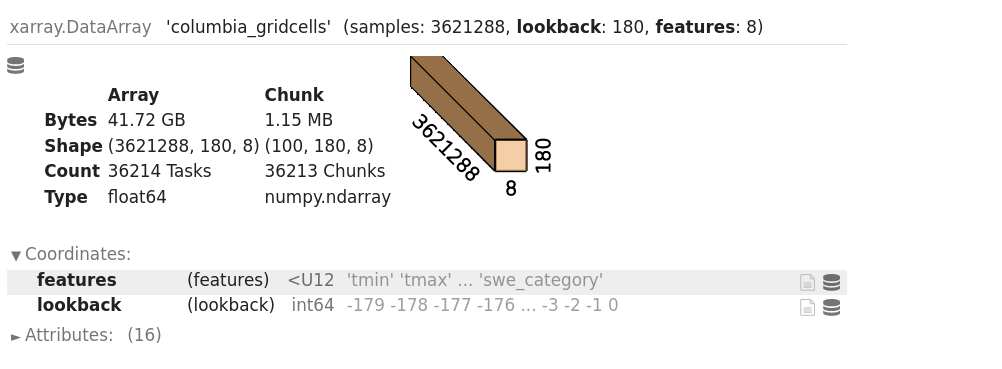
Let’s take a moment to reflect on how cool this actually is. You’ve just opened up a very large dataset stored on one machine over the network to another machine in a very small number of lines of code, and you retain the labels and metadata of your data. So now the question about how to reasonably access this data over the network.
As xarray loads data lazily, now you will need to figure out how to get the data across the network in an efficient an automated manner. This is largely going to depend on how your data is aranged/formatted, and is beyond the scope of this post. But, you now have the tools you need to load the data across the network.