Historical Motivation

Marcus Vitruvius is often credited with some of the earliest attributed treatises on the description of the water cycle over terrestrial environments (Raffensperger, 2014). His recognition that water in the subsurface is derived from precipitation and infiltration rather than upwelling from subterranean aquifers allowed for insights that allowed civilizations throughout history access to stable sources of water. Some 2000 years later the exact details of these infiltration processes still escape mankind’s ability to fully explain, though considerable progress has been made on several avenues. A major contribution to the understanding of hydrological processes was determined experimentally in the mid ninteenth century by the French engineer Henri Darcy. When comissioned to help design a water treatment system he found that no suitable description of the flow through a porous media existed. Darcy’s experiments were conducted by packing a tube with sand of estimable diameter, and it’s effect on the flow through the cylinder was measured and related to the loss of hydraulic pressure over some distance. His experiments derived what became known as Darcy’s Law.

Coincidentally, it was roughly the same time that Claude Navier and George Stokes (amongst others) were working on what would become to be known as the Navier-Stokes equations. It took more than 200 years from the time of Darcy, Navier, and Stokes to show that Darcy’s law could be derived directly from the Navier-Stokes equations. This work was accomplished as late as 1986 as shown in (Whitaker, 1986). Soon following this the result that this paper finds itself concerned with was developed. Lewis Richardson (and subsequently Lorenzo Richards, for which the equation gained its namesake) provided an extension of Darcy’s law which describes the flow of fluids in unsaturated porous media. His formulation of these flows has been increasingly subjected to numerical analysis as computing power has increased, though many methods have been shown to be lacking due to various causes. This paper represents an attempt to understand the challenges and shortcomings of numerical approaches to solving Richards’ equations in simplified environments.

Overview of governing equations

Darcy’s Law

Darcy’s law describes the flow of a fluid in a saturated porous medium. That is, pores between solid granules are completely filled with the liquid. The flow of some arbitrary parcel of fluid may be highly complex, and it would have been an untractable problem during the time of Darcy (and in most ways, still is). Instead, if the size of the domain of interest is much greater than the grain size found within the system we can obtain a first order approximation to the system by assuming some bulk behavior of the fluid through the medium. Darcy’s experiments and analysis provided one such approximation that thas shown to be quite useful in hydrological science and engineering applications.

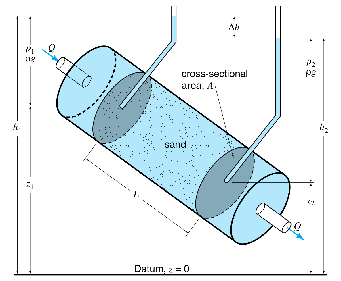
The experimental setup for the experiments conducted by Henri Darcy is shown in figure 1. In his experiments he measured the discharge, \(Q (m^3/s)\), and the change in hydraulic pressure head, \(H(m)\), due to friction and turbulence. He found that the total discharge was directly proportional to the hydraulic head loss over some distance. Written generally, Darcy’s law in one dimension is given by

where \(K (m/s)\) is a constant known as the hydraulic conductivity. This quantity represents the ease with which a liquid can flow through a medium, much as its electromagnetic analogue describes the ability for current to flow.

Richards’ Equation

Darcy’s law can be extended to unsaturated conditions by recognizing that the hydraulic conductivity is affected by amount of saturation. This amount can be quantified by the fractional moisture content \(\theta\). The values for \(\theta\) are between 0 (for fully dry) and 1 (for fully saturated). Thus we have Darcy’s law for unsaturated media

where the function \(K(\theta)\) is material dependent. To track how fluid moves throughout a medium we would be concerned with knowing the value for \(\theta\) throughout time. The resulting equation is what is known as Richards’ equation. In order to derive it we must recognize one more fact; the hydraulic pressure head, \(H\), can be broken into two components. We say

where \(h\) is the capillary pressure head, caused by surface tension and adhesion, and \(z\) is the elevation head. Note that \(h\) is a function of the moisture content.

Using this fact we can rewrite Darcy’s law

Now we use the continuity relation

to obtain Richards’ equation

This form of the equation is known as the mixed form, two additional forms are popular in the literature as well

where \(C(h) = \frac{d\theta}{dh}\). And,

Finite difference discretizations

Fully explicit first order method

We can discretize both the mixed and head based versions of Richards equation using an explicit Euler scheme. The resulting methods are

for the mixed form and

for the head based form. Both forms use an averaged hydraulic conductivity which was given in Zarba, 1988 and has the form

Implicit first order method with Picard iteration

To develop a more robust approximation we can use the backward Euler method to discretize the head-based formulation. The resulting method is

Because of the general nonlinearity of this system solutions must be sought in an iterative manner. Picard iteration (or the application of fixed point iteration) is a relatively simple method that serves as a good baseline for solving the implicit system. We denote the \(m-th\) iteration for a variable \(X\) as \(X_j^{n, m}\). Then the Picard iterative solution can be found by applying

We can simplify the next step by defining \(\delta h_j^{n+1, m} \equiv h_j^{n+1, m+1} - h_j^{n+1, m}\). Then, grouping terms leads us to

This system can be written much more concisely as

Where \(\hat{A}\) is a tridiagonal matrix given by

where

A solution can be reached by iterating on this equation until some desired residual tolerance is met for \((\vec{\delta h}^{n+1,m})\).

Implicit first order method with modified Picard iteration

Despite more advanced iterative techniques, such as Newton’s method, it was discovered that such formulations (including the simple Picard iteration) do not conserve mass suitably well. As modern hydrological models are built off of the assumptions of mass and energy conservation, this becomes a problem for models that are based on the finite difference method. Unfortunately, it has been the case that the majority of these models are built upon finite differencing for some time, and will be for the forseable future.

It was with this realization that Zarba, 1988 introduced the modified Picard iteration method for this application, which was shown to have better mass conservation properties than the standard Picard iteration and Newton iteration methods have.

To derive this method we first provide the backward Euler discretization of the mixed equation

Following the same path as the previously discussed method we can set up the iteration

At this point we replace the updated fractional moisture content with a Taylor series expansion

Dropping the higher order terms and substituting this back in we have

Recognizing that \(\frac{d\theta}{dh} = C\), we can substitute in and then following from the previous process by grouping terms and simplifying we find

Where our system, again, can be written much more concisely as

Where the left hand side is identical to the standard Picard iterative method, but the right and side has a different first term. As before, our approximation can be reached by iterating on this equation until some error tolerance has been met.

A naive approach to adaptive mesh refinement

Finally, we also introduce a naive approach to adaptive mesh refinement. We will apply this method only the the explicit formulations due to the ease of implementation. We should note that it would be inadvisable to apply this method to the modified Picard iteration scheme, as it makes almost no guarantees about conserving mass in any sane ways. All mentions of regridding are accomplished via linear interpolation.

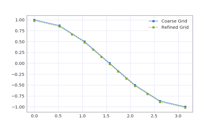
The algorithm developed for mesh refinement is as follows. First, input data is regridded onto a default grid that is unchanging throughout time. This was taken to be the initial grid for all experiments. Then, the discrete gradient was taken by calculating the slope between each pair of grid points. This set of slopes is then normalized to some value that represents the maximum number of new grid points between any two existing grid points. For all experiments this was arbitrarily set to 2, to avoid artifacts. This normalized slope factor array contains the number of new grid points that should be assigned to the range.

The new grid is then developed from this information, and the updated solution is obtained from regridding the initial dataset to the new one. A simple example of the procedure is shown in figure 2.

Results

Due to the highly nonlinear nature of Richards’ equation analytical solutions can only be derived for highly simplified cases. We will look at the numerical solutions to a case described in Celia et. al, 1990 and VanGenuchten, 1980. First, we will look at the problem setup as described in VanGenuchten, 1980. Despite the name of the paper, the closed form was determined as a method of fitting curves to empirical data. Despite the fact that no verification or validation data exists this setup does have some advantages for exploration. One important fact of this system is that the \(\theta - h\) relationship is invertible, which makes the head-based explicit formulation simple to implement.

The setup is as follows

\(\theta(h) = \frac{\theta_s - \theta_r}{(1+(a h)^n)^m} + \theta_r\) \(K(h) = K_s \frac{1 - (ah)^{n-2}(1+(ah)^n)^{-m}}{(1+(ah)^n)^{2m}}\)

where \(a=0.0335\), \(\theta_s=0.368\), \(\theta_r=0.102\), \(n=2\), \(m=4\) and \(K_s=0.00922 cm/s\). Initial boundary conditions are given as \(h(z,0)=-1000cm\), \(h(0,t) = -1000cm\), \(h(60, t) = -75cm\).

Three runs were conducted to show the behavior of the explicit methods. These runs were carried out to \(t_{end} = 3600s\) with 24 nodes in the grid. The results are shown in figures 3 and 4.

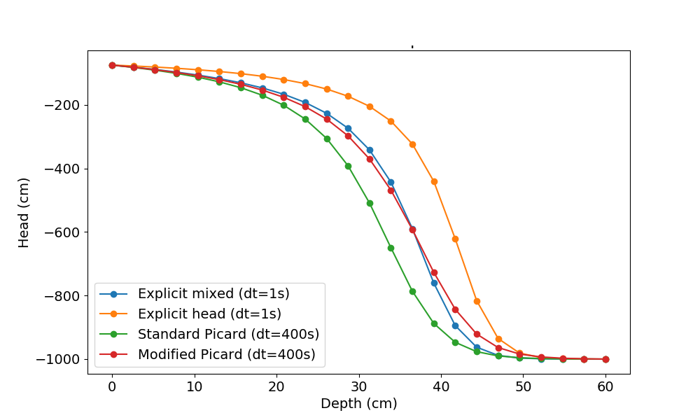
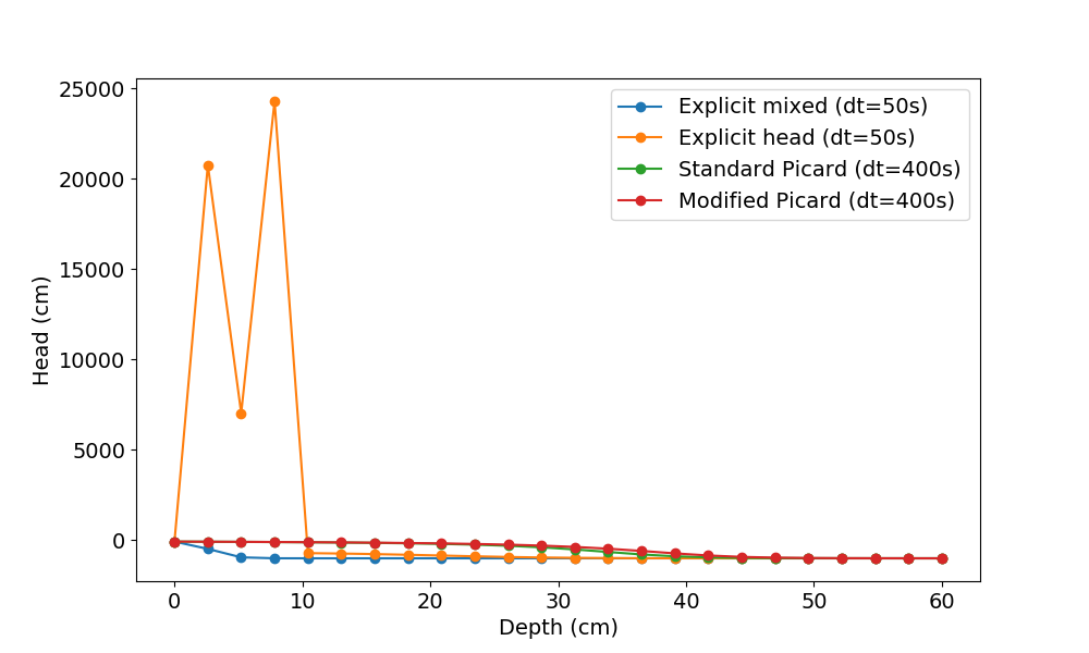
As we can see from these simple experiments the explicit methods, and especially the head-based formulation, have rather large issues. Because of this we exclude them from some of the future analyses. Before looking exclusively at the implicit methods, though, we would like to see if any gains can be made in the explicit methdods by using the simple mesh refinement algorithm discussed above.

Adaptive mesh

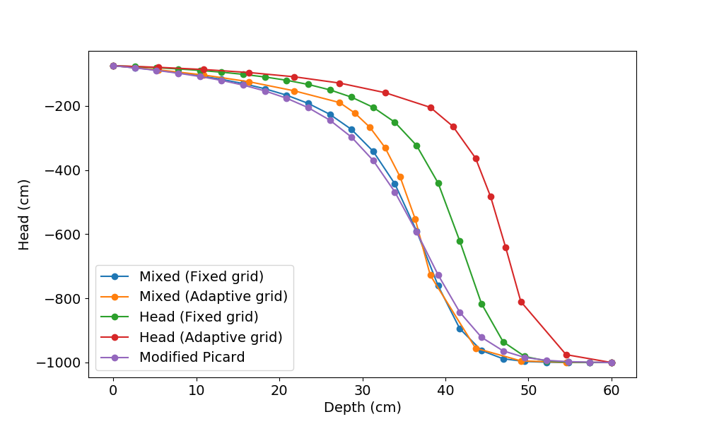
Figure 5 shows a comparison of the explicit methods with adaptive regridding every 360s. It can be seen evidently that the adaptive methods advanced the wetting front more quickly than their non-adaptive counterparts. This is not in line what is seen in the implicit method, so this method will be left as an avenue for further exploration in the future.

Mass balance in the implicit methods

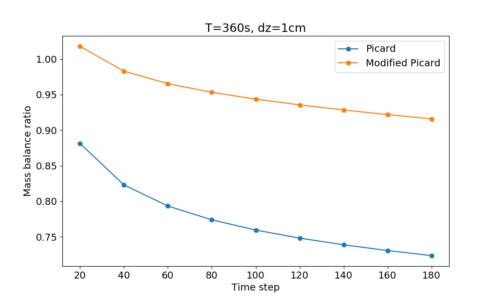
The mass balance equation can be derived from the continuity equation and is provided in Celia et al, 1990 as

This quantity was calculated for several timesteps with a final time of 360 seconds. As shown in figure 6 the modified Picard iteration method has much better mass conservation properties.

Validation

Despite the fact that no closed form exists for this case we can validate the model that was developed above by using a benchmark solution. According to Oberkampf and Roy, 2010 the purpose of validation is to build credibilty, thus we use an appeal to authority.

The Structure for Unifying Multiple Modeling Alternatives (SUMMA) Clark et. al, 2015 is a hydrological model developed by the National Center for Atmospheric Research (NCAR). It is built on a core that consists of the base conservation equations and a common numerical solver upon which different physics can be implemented. One of the test cases for SUMMA is an implementation of the problem described below, using the method used by Zarba, 1988 (which we called the modified Picard method).

The case that is implemented in SUMMA is the second experiment performed in Celia et. al, 1990, which was derived from conversations with D. Polmann. Unfortunately, verification data for this does not exist either. Overall, the setup is similar to that which was explored above, but with a sharper wetting front. The problem is described as follows

\(\theta(h) = \frac{\theta_s - \theta_r}{(1+(a h)^n)^m} + \theta_r\) \(K(h) = K_s \frac{((1-(a h)^{n-1}(1+(a h)^n)^{m/2})^2}{(1+(a h)^n)^{m/2}}\)

where \(a=0.0335\), \(\theta_s=0.368\), \(\theta_r=0.102\), \(n=2\), \(m=0.5\) and \(K_s=0.00922 cm/s\). Initial boundary conditions are given as \(h(z,0)=-1000cm\), \(h(0,t) = -1000cm\), \(h(60, t) = -75cm\).

Simulations were run at a timestep of \(\Delta t = 2800s\), which eliminates the practical usage of the explicit methods (and thus, the ad hoc adaptive routine). The grid spacing matched the test case in SUMMA, with 100 grid cells over a depth of 60 cm. Running these simulations, we can compare our results to the SUMMA test output. The results can be seen in figure 7.

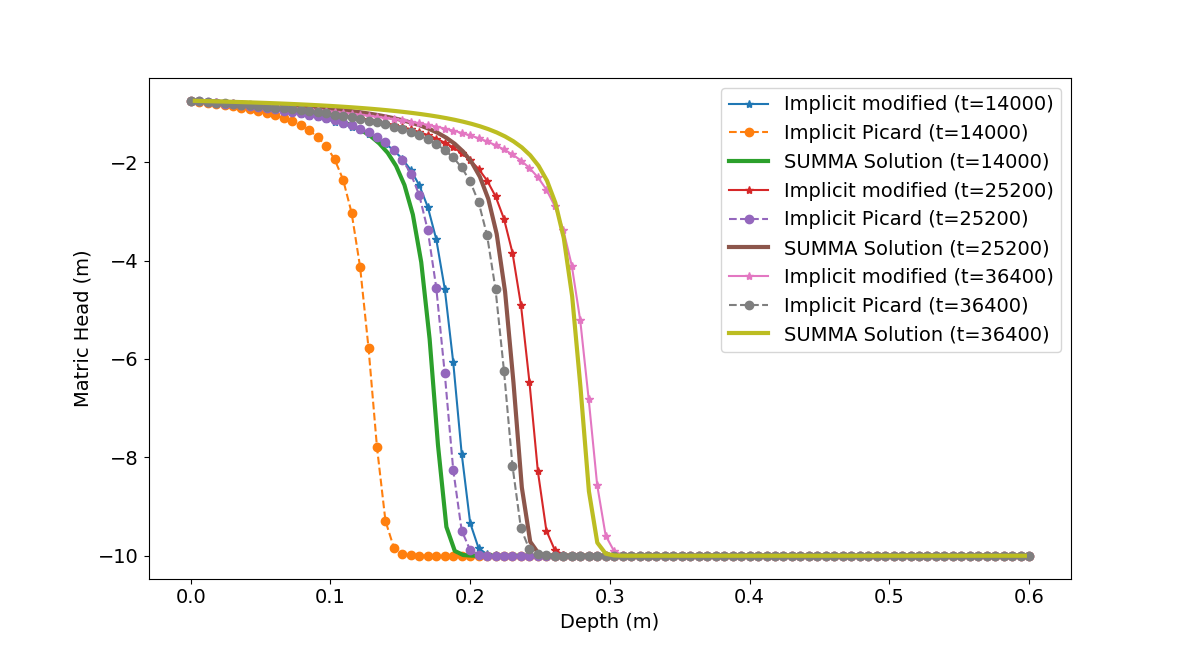
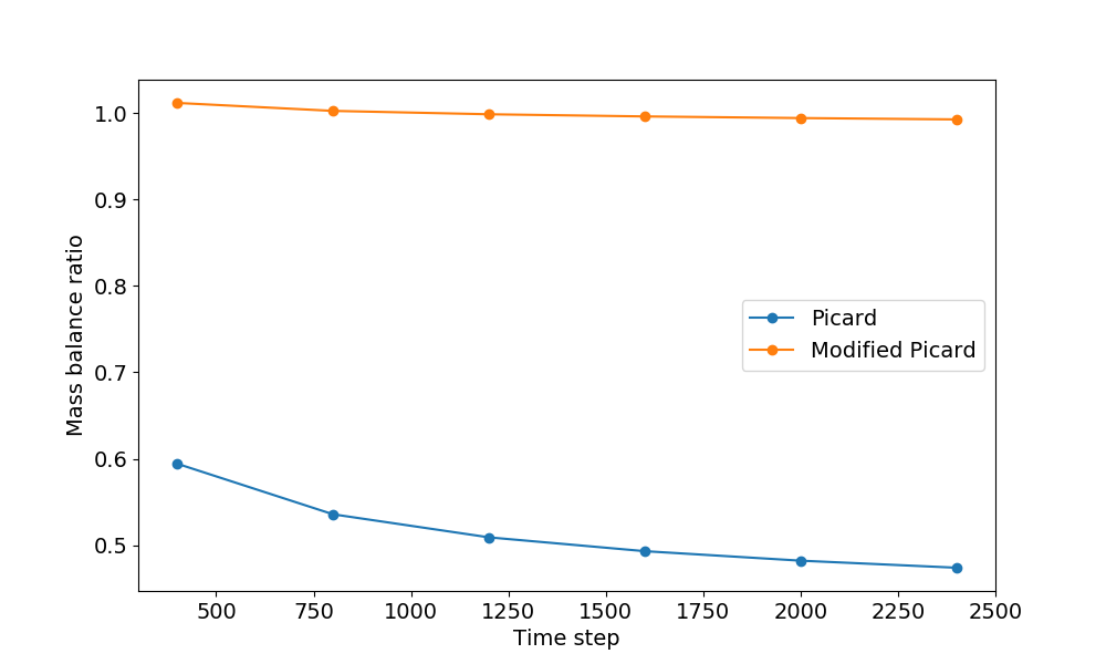
We can see that the standard Picard iteration did significantly worse than the modified Picard method for this case, as compared to the SUMMA simulation. It seems reasonable that this deficiency is due to the unfavorable mass balance ratio we have seen previously. Figure 8 builds confidence in this hypothesis.

Given the results thus far, it is reasonable to conclude that the modified Picard is the overall best method developed here. It still may be useful to know how our implementation stacks up against the method that is implemented in SUMMA. Shown in figure 9 is the RMSE calculated over time for this setup.

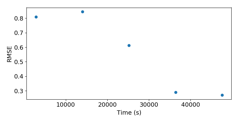
We can see that the error drops over time as shown in figure 10, it appears that this is mostly a compensatory error by examining figure 11. It seems that it may be worthwile to run both simulations at finer timesteps, and for longer periods to gain a better understanding of the true relationship between the solutions.

Conclusions

We have examined four methods of discretization of Richards’ equation, and two test cases. We have seen that first order explicit methods are unsuitable for even the simplest of problems, and should favor more stable methods that allow for greater timesteps. In this overview we have only examined first order methods. Initially it was the author’s intent to explore higher order methods, but because there were no suitable analytical test cases this avenue was not initially pursued. The brief review of the literature suggests that first order methods are a common approach. It seems likely that this is because in hydrological disciplines the input data has a higher uncertainty than even errors introduced via first order approximation. Indeed, this is the stance taken in Beven and Cloke, 2012.

The adaptive scheme briefly attempted here does, however, show some promise even though initial results were quite poor. It seems reasonable that the poor results were because the method discretized on where the gradient was highest, rather than attempting to predict the areas that the gradient would be highest until the next regridding. An avenue for further research would be to attempt to incorporate this "grid-velocity" into an implicit method. It seems possible that some formulation could be adapted for the modified Picard iteration method which was most successful here but this is far beyond the scope of the work of this paper.

References

[1] Keith J. Beven and Hannah L. Cloke. Comment on hyperresolution global land surface modeling: Meeting a grand challenge for monitoring earth’s terrestrial water by eric f. wood et al. Water Resources Research, 48(1):n/a–n/a, 2012. W01801.

[2] Michael A. Celia, Efthimios T. Bouloutas, and Rebecca L. Zarba. A general mass-conservative numerical solution for the unsaturated flow equation. Water Resources Research, 26(7):1483– 1496, 1990.

[3] Martyn P. Clark, Bart Nijssen, Jessica D. Lundquist, Dmitri Kavetski, David E. Rupp, Ross A. Woods, Jim E. Freer, Ethan D. Gutmann, Andrew W. Wood, Levi D. Brekke, Jeffrey R. Arnold, David J. Gochis, and Roy M. Rasmussen. A unified approach for process-based hydrologic modeling: 1. modeling concept. Water Resources Research, 51(4):2498–2514, 2015.

[4] Jeffrey P. Raffensperger George M. Hornberger, Patricia L. Wiberg and Paolo D’Odorico. Ele- ments of Physical Hydrology. Johns Hopkins University Press, Baltimore, 2014.

[5] William L. Oberkampf and Christopher J. Roy. Verification and Validation in Scientific Com- puting. Cambridge University Press, New York, 2010.

[6] M Th Van Genuchten. A closed-form equation for predicting the hydraulic conductivity of unsaturated soils. Soil science society of America journal, 44(5):892–898, 1980.

[7] Stephen Whitaker. Flow in porous media i: A theoretical derivation of darcy’s law. Transport in Porous Media, 1(1):3–25, 1986.

[8] Rebecca Zarba. A numerical investigation of unsaturated flow. Master’s thesis, Massachusetts Institute of Technology. Dept. of Civil Engineering., Massachusetts Institute of Technology, 1988.