Can a neural network play Conways Game of Life?
TL;DR: Yes!
Getting started
After cleaning up the notebook from my previous post on SineNets I wanted to
explore a slightly more complicated system, but still what would be considered
pretty simple as far as machine learning goes: Conway’s Game of Life.
I’m not really going to get into the description or background, so if you want to learn more check the Wikipedia link.
To see if a simple convolutional neural network can learn the kernel for Game of Life (GOL, hereafter) we first
need a baseline implementation. This is easy enough to do with scipy.signal.convolve2d, which conveniently enough
also makes it explicit what the kernel values are that the network needs to learn, more or less. Note that the network
won’t have to simple learn the values in kernel but also the update rules in the to_kill, to_live, and to_born
variables of the update function, gol_update. I also implemented a looped simulation in gol_simulate and an animation function to save some time later.
import numpy as np
import matplotlib.pyplot as plt
import matplotlib.animation as animation
import scipy.signal
import torch
from torch import nn
import torch.nn.functional as F
import pytorch_lightning as pl
np.random.seed(42)
DEVICE = torch.device("cuda:0" if torch.cuda.is_available() else "cpu")

SIZE = (64, 64)
INIT_FRAC = 0.4
BURN_IN_STEPS = 5
N_SAMPLES = 1_000
EPS = 1e-5

def gol_update(grid):
    kernel = np.array([
        [1, 1, 1],
        [1, 0, 1],
        [1, 1, 1]
    ])
    neighbors = scipy.signal.convolve2d(grid, kernel, mode='same')
    new_grid = np.zeros_like(grid)
    to_kill = np.logical_or(neighbors < 2, neighbors > 3)
    to_live = np.logical_and(
        np.logical_or(neighbors == 2, neighbors == 3),
        grid == 1
    )
    to_born = neighbors == 3
    new_grid[to_kill] = 0
    new_grid[to_live] = 1
    new_grid[to_born] = 1
    return new_grid

def gol_simulate(grid, steps):
    simulation = []
    for _ in range(steps):
        grid = gol_update(grid)
        simulation.append(grid)
    return np.stack(simulation)

def save_animation(frames, filename):
    fig, ax = plt.subplots(1, 1, dpi=100)
    ims = []
    for f in frames:
        im = ax.imshow(f, interpolation='nearest', animated=True)
        ax.set_xticks([])
        ax.set_yticks([])
        ims.append([im])

    ani = animation.ArtistAnimation(fig, ims, interval=5, blit=True,
                                    repeat_delay=10)
    ani.save(filename)
Getting the data together for training the model
Of course, with any machine learning problem, getting the data prepared is half the battle, and so
here I implemented a routine to generate a single sample, generate_sample. The goal is to take in
an input map, and simply try to output the next generation (ie what would come out if we ran gol_update).
But, to avoid initialization “noise” I actually run the simulation for some number of burn_in_steps just
to make the samples more representative of what GOL actually looks like. Following that I make a function
to create many samples and a GOLDataset class to make it official.
def generate_sample(
    size=SIZE,
    init_frac=INIT_FRAC,
    burn_in_steps=BURN_IN_STEPS
):
    """Create a sample of input/output for GOL training"""
    x = np.random.random(size) < init_frac
    for _ in range(burn_in_steps):
        x = gol_update(x)
    y = gol_update(x)
    return x, y

def generate_data(
    size=SIZE,
    init_frac=INIT_FRAC,
    burn_in_steps=BURN_IN_STEPS,
    n_samples=N_SAMPLES
):
    """Create a set of training data for GOL"""
    xs = []
    ys = []
    for _ in range(n_samples):
        x, y = generate_sample(size, init_frac, burn_in_steps)
        # Note the [listing] to get a "channel" dimension when
        # we do the stack at the end for nn.Conv2d convention
        xs.append([x])
        ys.append([y])
    return np.stack(xs), np.stack(ys)

class GOLDataset(torch.utils.data.Dataset):
    def __init__(self, x, y):
        self.x = torch.tensor(x, dtype=torch.float32).to(DEVICE)
        self.y = torch.tensor(y, dtype=torch.float32).to(DEVICE)

    def __len__(self):
        return len(self.x)

    def __getitem__(self, i):
        return self.x[i], self.y[i]
With all of the functions/classes together for data preparation I generate soem training, validation, and testing data.
This is all pretty straightforward. Note we’ll train on (64, 64) pixel grids but on the test data I’ll make it much bigger, a (256, 256) pixel grid. This just makes the animations at the end cooler.
n_train = 10_000
n_valid = 3_000
n_test  =  10
xtrain, ytrain = generate_data(n_samples=n_train)
xvalid, yvalid = generate_data(n_samples=n_valid)
xtest, ytest = generate_data(n_samples=n_test, size=(128, 128))

train_dl = torch.utils.data.DataLoader(
    GOLDataset(xtrain, ytrain),
    batch_size=256,
    num_workers=0,
    shuffle=True
)

valid_dl = torch.utils.data.DataLoader(
    GOLDataset(xvalid, yvalid),
    batch_size=256,
    num_workers=0
)

test_dl = torch.utils.data.DataLoader(
    GOLDataset(xtest, ytest),
    batch_size=1,
    num_workers=0
)
Model time
To define the model, I’m just using about the simplest CNN you can possibly use. I expand to a configurable number of hidden channels, ReLU that, and then contract it back down to a single channel, followed by a sigmoid to scale things on 0-1. I’m using pytorch-lightning here to
make the training loop simpler, although to pull out the loss curves for this notebook I need to implement a callback to log them, rather than going to TensorBoard. I’m really on the fence if this was actually easier/faster than just writing my own training loop.
In the GameOfLifeCNN I set the optimizer to Adam (as is customary) and the loss to be binary cross entropy since this is a binary problem.
class MetricsCallback(pl.Callback):
    """Just to make pulling out the logs easier"""
    def __init__(self):
        super().__init__()
        self.metrics = {'train_loss': [], 'valid_loss': []}

    def on_validation_epoch_end(self, trainer, pl_module):
        each_me = copy.deepcopy(trainer.callback_metrics)
        for k, v in each_me.items():
            self.metrics[k].append(v.cpu().detach().numpy())


class GameOfLifeCNN(pl.LightningModule):

    def __init__(
        self,
        hidden_dim,
        kernel_size=3,
    ):
        super().__init__()
        self.padding = int(kernel_size/2)
        self.model = nn.Sequential(
            nn.Conv2d(1, hidden_dim, kernel_size, padding=self.padding),
            nn.ReLU(),
            nn.Conv2d(hidden_dim, 1, kernel_size, padding=self.padding),
            nn.Sigmoid()
        )

    def forward(self, x):
        return self.model(x)

    def configure_optimizers(self):
        optimizer = torch.optim.Adam(self.parameters(), lr=1e-2)
        return optimizer

    def training_step(self, train_batch, batch_idx):
        x, y = train_batch
        yhat = self.forward(x)
        loss = F.binary_cross_entropy(yhat, y)
        self.log('train_loss', loss)
        return loss

    def validation_step(self, val_batch, batch_idx):
        x, y = val_batch
        yhat = self.forward(x)
        loss = F.binary_cross_entropy(yhat, y)
        self.log('valid_loss', loss)

    def simulate(self, x, n_steps):
        simulation = []
        for _ in range(n_steps):
            with torch.no_grad():
                x = self.forward(x)
                simulation.append(x.detach().cpu().numpy().squeeze())
        return np.stack(simulation)
Training the simplest possible model
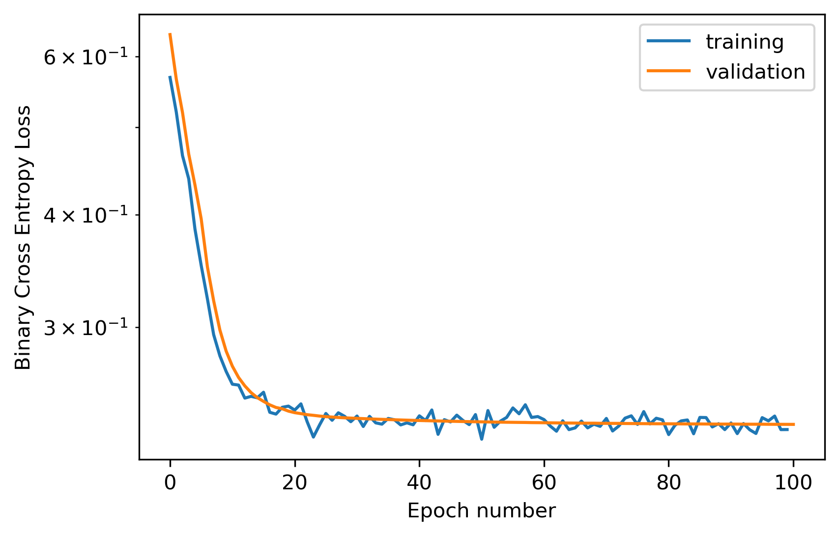
First thing to do is try to train the simplest model we can, so we set hidden_dim to 1 and let it train for 100 epochs. We can see the loss levels out after ~40 epochs with a value of something like 0.25 or so. But is it good enough?
max_epochs = 100
c = MetricsCallback()

model = GameOfLifeCNN(hidden_dim=1).to(DEVICE)
trainer = pl.Trainer(gpus=1, max_epochs=max_epochs, callbacks=[c], progress_bar_refresh_rate=0)
trainer.fit(model, train_dl, valid_dl, )

fig, ax = plt.subplots(1, 1, dpi=300)
plt.plot(c.metrics['train_loss'], label='training')
plt.plot(c.metrics['valid_loss'], label='validation')
plt.semilogy()
plt.legend()
plt.xlabel('Epoch number')
plt.ylabel('Binary Cross Entropy Loss')
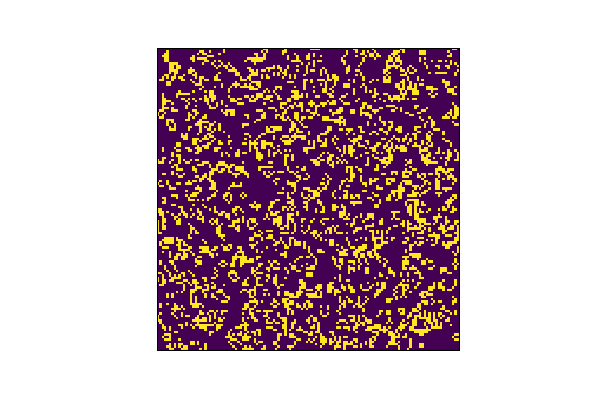
To find out, let’s run the model on some test data. I’ll just let the thing simulate out 100 timesteps. As a comparison I’ve also gone ahead and simulated the same starting point for 100 timesteps. First, let’s look what comes out of the true Game of Life simulation. It looks as you might expect if you’ve seen Game of Life before.
model = model.to(DEVICE)
x, y = next(iter(test_dl))
sim_steps = 100
out_hat = model.simulate(x, sim_steps)

x_init = x.cpu().detach().squeeze().numpy()
out_tru = gol_simulate(x_init, sim_steps)
save_animation(out_tru, 'gol_truth.gif')

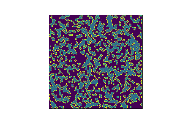
But, the CNN version… not so much. It does look pretty cool though. Almost like a jagged run of the Ising Model, which I might explore later.
save_animation(out_hat, 'gol_cnn_bad_fit.gif')
Can we do better?
Given the TL;DR, obviously. And it turns out it’s not actually that hard to do. Bumping up the hidden_dim to 3 does the job. I only ran 100 epochs, but you can see the loss still dropping quite quickly. I just let it run out there because this seems to do the trick on forward simulations.
max_epochs = 100
c = MetricsCallback()

model = GameOfLifeCNN(hidden_dim=3).to(DEVICE)
trainer = pl.Trainer(gpus=1, max_epochs=max_epochs, callbacks=[c], progress_bar_refresh_rate=0)
trainer.fit(model, train_dl, valid_dl, )

fig, ax = plt.subplots(1, 1, dpi=300)
plt.plot(c.metrics['train_loss'], label='training')
plt.plot(c.metrics['valid_loss'], label='validation')
plt.semilogy()
plt.legend()
plt.xlabel('Epoch number')
plt.ylabel('Binary Cross Entropy Loss')
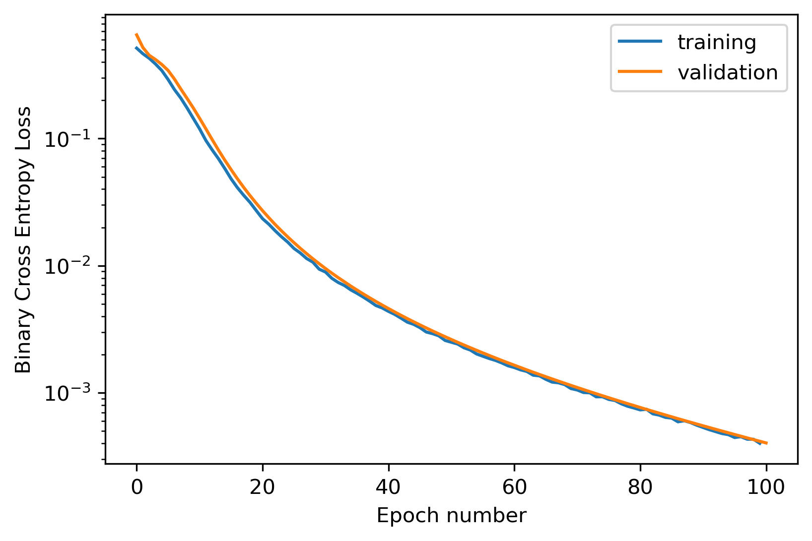
Without further adieu, a neural network Game of Life simulation. Looks pretty good. I’ve actually run these out to 1000+ steps and it’s pretty stable. I’ve also trained the thing out much further and you can essentially get the loss to be within numerical tolerance, which basically means the problem is fully solved. That’s, that!
model = model.to(DEVICE)
out_hat = model.simulate(x, sim_steps)
save_animation(out_hat, 'gol_cnn_good_fit.gif')