Been thinking about this twitter post a bit this week and wanted to give a few things a try. Originally I wanted to design a neural net with off the shelf components and no special tricks (like taking inputs modulo pi or fitting on the Fourier transform). This is a surprisingly hard thing to get a neural network to learn. This made me wonder, can we just get the neural network to learn the frequency multiplier in the sine function itself. Starting there, let’s do some imports…

%pylab inline
import matplotlib as mpl
import torch
import torch.nn as nn
import torch.nn.functional as F
from tqdm.notebook import tqdm
device = torch.device("cuda:0" if torch.cuda.is_available() else "cpu")

# Set a bigger default plot size
mpl.rcParams['figure.figsize'] = (12, 8)
mpl.rcParams['font.size'] = 22

Setting up the initial experiment

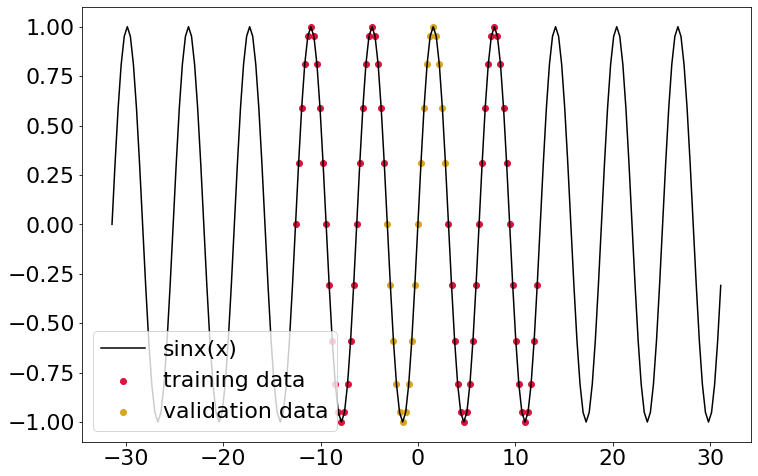
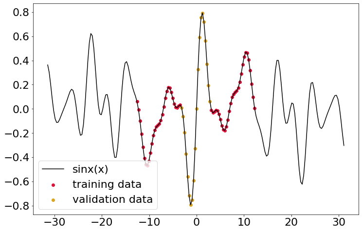
Here I’ll make some true data (a basic sine wave), and pick out some discontinuous section for training data, along with a bit of validation data. The plot below gives the situation.

dtype = torch.float32
dx = 0.01
x_train = torch.hstack([
    torch.tensor(np.pi * np.arange(-12.0, -1.0, step=dx), dtype=dtype),
    torch.tensor(np.pi * np.arange(1.0, 12.0, step=dx), dtype=dtype),
])
y_train = np.sin(x_train)

dtype = torch.float32
dx = 0.1
x_train = torch.hstack([
    torch.tensor(np.pi * np.arange(-4.0, -1.0, step=dx), dtype=dtype),
    torch.tensor(np.pi * np.arange(1.0, 4.0, step=dx), dtype=dtype),
])
x_valid = torch.tensor(np.pi * np.arange(-1, 1, step=dx), dtype=dtype)
y_train = torch.sin(x_train)
y_valid = torch.sin(x_valid)

x_truth = np.pi * np.arange(-10, 10, step=dx)
y_truth = np.sin(x_truth)

plt.plot(x_truth, y_truth, color='black', label='sinx(x)')
plt.scatter(
    x_train, y_train,
    color='crimson', marker='o', label='training data'
)
plt.scatter(
    x_valid, y_valid,
    color='goldenrod', marker='o', label='validation data'
)
plt.legend(loc='lower left')

png

The definition of the `SineNet` network

Okay, great, now to define a network which takes a width parameter (which determines the number of trainable parameters) that will be used to compute:

\[y = \frac{1}{width} \sum_{i=0}^{width} sin(\pi \cdot w_i \cdot x)\]

This is a clearly very strong inductive bias in learning the right function so it should be no problem to get a nearly perfect fit. Right?

class SineNet(nn.Module):
    def __init__(self, width):
        super().__init__()
        self.w = nn.Parameter(2 * torch.rand(width), requires_grad=True)

    def forward(self, x):
        pi = torch.tensor(3.14159)
        # Mean to keep outputs [-1 1]
        return torch.mean(torch.sin(pi * self.w * x))

Before getting there - one more definition, our training epoch. Nothing special is going on in here.

def epoch(
    X, y,
    model,
    loss_fun,
    device=device,
    opt=None,
    monitor=None,
    X_valid=None,
    y_valid=None,
):
    total_loss, total_err, total_monitor = 0.,0.,0.
    model.eval() if opt is None else model.train()
    n_iter = X.shape[0]
    for i in range(n_iter):
        Xd, yd = X[[i]].to(device), y[[i]].to(device)
        if opt:
            opt.zero_grad()
        yp = model(Xd / np.pi)
        loss = loss_fun(yp, yd) #, yp_prime, yd_prime)
        if opt:
            loss.backward()
            if sum(torch.sum(torch.isnan(p.grad)) for p in model.parameters()) == 0:
              opt.step()
        total_loss += loss.item() * X.shape[0]
        if monitor is not None:
            total_monitor += monitor(model)

    total_val_loss = 0.0
    if X_valid is not None:
        n_iter = X_valid.shape[0]
        for i in range(n_iter):
            Xd, yd = X_valid[[i]].to(device), y_valid[[i]].to(device)
            yp = model(Xd / np.pi)
            loss = loss_fun(yp, yd)
            total_val_loss += loss.item() * X_valid.shape[0]
            if monitor is not None:
                total_monitor += monitor(model)
    return total_loss / len(X), total_val_loss / len(X_valid)

Training

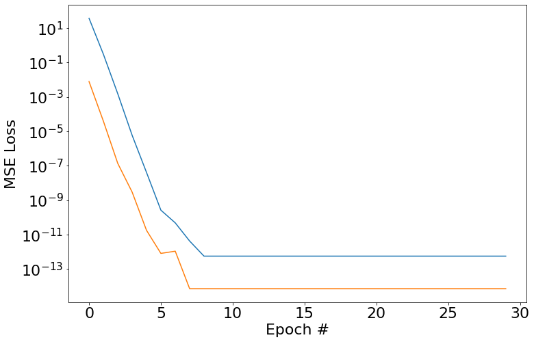
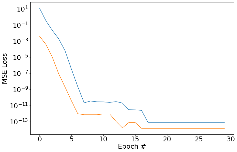
So here we go, we set a width of 1 since we only have one frequency in the generated training data. As you can see, we fit this no problem.

width = 1
model = SineNet(width)
loss_fun = torch.nn.MSELoss()
opt = torch.optim.Adam(model.parameters(), lr=0.01)

train_loss_history = []
valid_loss_history = []

max_epochs = 30
for i in tqdm(range(max_epochs)):
    train_loss, valid_loss = epoch(
        x_train,
        y_train,
        model,
        loss_fun,
        opt=opt,
        X_valid=x_valid,
        y_valid=y_valid
    )
    train_loss_history.append(train_loss)
    valid_loss_history.append(valid_loss)

plt.semilogy(train_loss_history)
plt.semilogy(valid_loss_history)
plt.xlabel('Epoch #')
plt.ylabel('MSE Loss')

png

Plotting this thing out of range

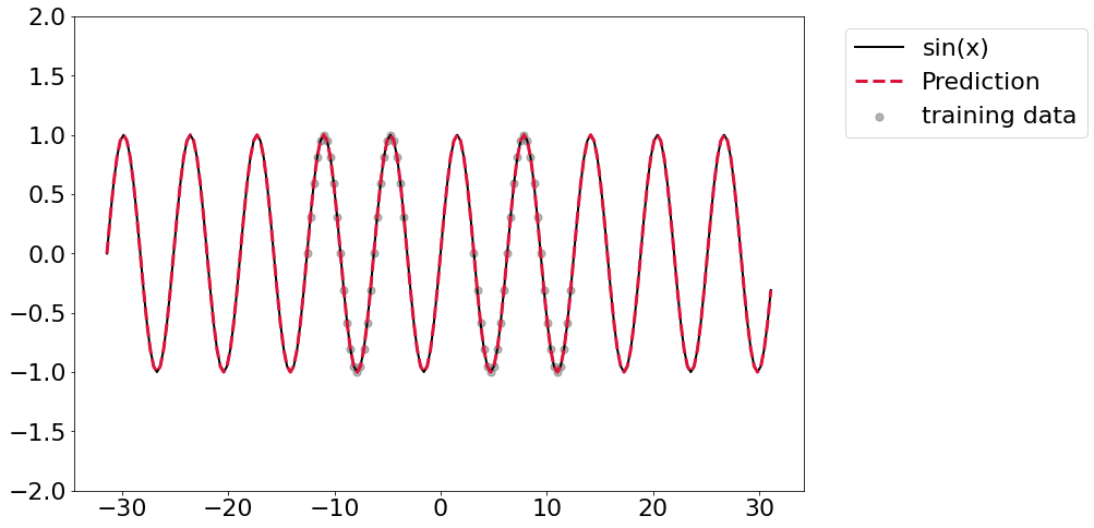
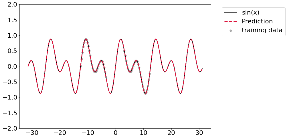
As the fit indicates, we can get really nice out of distribution prediction. We essentially learned the right function here.

y_pred = []
for x in x_truth:
    y_pred.append(model(torch.tensor([x/np.pi], dtype=dtype).flatten()).detach().numpy())

plt.plot(x_truth, y_truth, linewidth=2, color='black', label='sin(x)')
plt.scatter(x_train, y_train, color='grey', marker='.', alpha=0.6, s=200, label='training data')
plt.plot(x_truth, np.hstack(y_pred), linewidth=3, color='crimson', linestyle='--', label='Prediction')
plt.ylim([-2,2])
plt.legend(bbox_to_anchor=(1.04,1), loc="upper left")

png

Now for something a bit more complicated…

Let’s make use of that width parameter and try to learn a linear superposition of two sine waves. I’ll just manually set the coefficients here. And then train with width=2 on the SineNet. Again, we can pretty easily learn this. If you run this code it might take a couple of tries to get convergence, but it should be pretty straightforward to get it to happen.

Again we get that really nice prediction out of range.

y_truth = (np.sin(x_truth / 2) + np.sin(x_truth ))/2

dtype = torch.float32
dx = 0.1
x_train = torch.hstack([
    torch.tensor(np.pi * np.arange(-4.0, -1.0, step=dx), dtype=dtype),
    torch.tensor(np.pi * np.arange(1.0, 4.0, step=dx), dtype=dtype),
])
x_valid = torch.tensor(np.pi * np.arange(-1, 1, step=dx), dtype=dtype)
y_train = (torch.sin(x_train / 2) + torch.sin(x_train ))/2
y_valid = (torch.sin(x_valid / 2) + torch.sin(x_valid ))/2

plt.plot(x_truth, y_truth, color='black', label='sinx(x)')
plt.scatter(x_train, y_train, color='crimson', marker='o', label='training data')
plt.scatter(x_valid, y_valid, color='goldenrod', marker='o', label='validation data')
plt.legend(loc='lower left')

width = 2
model = SineNet(width)
#loss_fun = sobolov_loss#torch.nn.MSELoss()
loss_fun = torch.nn.MSELoss()
opt = torch.optim.Adam(model.parameters(), lr=0.01)

train_loss_history = []
valid_loss_history = []

max_epochs = 30
for i in tqdm(range(max_epochs)):
    train_loss, valid_loss = epoch(
        x_train,
        y_train,
        model,
        loss_fun,
        opt=opt,
        X_valid=x_valid,
        y_valid=y_valid
    )
    train_loss_history.append(train_loss)
    valid_loss_history.append(valid_loss)

plt.semilogy(train_loss_history)
plt.semilogy(valid_loss_history)
plt.xlabel('Epoch #')
plt.ylabel('MSE Loss')

png

y_pred = []
for x in x_truth:
    y_pred.append(model(torch.tensor([x/np.pi], dtype=dtype).flatten()).detach().numpy())

plt.plot(x_truth, y_truth, linewidth=2, color='black', label='sin(x)')
plt.scatter(x_train, y_train, color='grey', marker='.', alpha=0.6, s=200, label='training data')
plt.plot(x_truth, np.hstack(y_pred), linewidth=3, color='crimson', linestyle='--', label='Prediction')
plt.ylim([-2,2])
plt.legend(bbox_to_anchor=(1.04,1), loc="upper left")

png

Now for something way more complicated…

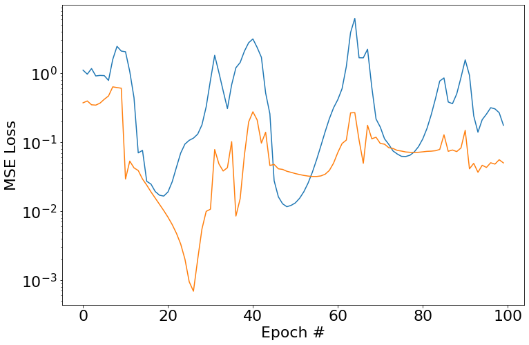
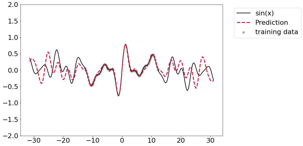
So obviously the next step is to keep bumping up width. Here I’ll randomly generate 8 coefficicents and split out the training and validation data as usual. This is where problems start to crop up - I’ve been unable to get this thing to converge. I’ve tried tinkering a bit with learning rates/number epochs/etc but it really doesn’t seem to want to get there. It does get reasonably close though, although the far ends of the prediction range aren’t great.

coefs = 2 * np.random.random(8)

y_truth = np.mean(np.array([np.sin(c * x_truth) for c in coefs]), axis=0)

dtype = torch.float32
dx = 0.1
x_train = torch.hstack([
    torch.tensor(np.pi * np.arange(-4.0, -1.0, step=dx), dtype=dtype),
    torch.tensor(np.pi * np.arange(1.0, 4.0, step=dx), dtype=dtype),
])
x_valid = torch.tensor(np.pi * np.arange(-1, 1, step=dx), dtype=dtype)
y_train = torch.tensor(np.mean(np.array([np.sin(c * x_train.numpy()) for c in coefs]), axis=0))
y_valid = torch.tensor(np.mean(np.array([np.sin(c * x_valid.numpy()) for c in coefs]), axis=0))

plt.plot(x_truth, y_truth, color='black', label='sinx(x)')
plt.scatter(x_train, y_train, color='crimson', marker='o', label='training data')
plt.scatter(x_valid, y_valid, color='goldenrod', marker='o', label='validation data')
plt.legend(loc='lower left')

png

width = 8
model = SineNet(width)
loss_fun = torch.nn.MSELoss()
opt = torch.optim.Adam(model.parameters(), lr=0.01)

train_loss_history = []
valid_loss_history = []

max_epochs = 100
for i in tqdm(range(max_epochs)):
    train_loss, valid_loss = epoch(
        x_train,
        y_train,
        model,
        loss_fun,
        opt=opt,
        X_valid=x_valid,
        y_valid=y_valid
    )
    train_loss_history.append(train_loss)
    valid_loss_history.append(valid_loss)

plt.semilogy(train_loss_history)
plt.semilogy(valid_loss_history)
plt.xlabel('Epoch #')
plt.ylabel('MSE Loss')

png

y_pred = []
for x in x_truth:
    y_pred.append(model(torch.tensor([x/np.pi], dtype=dtype).flatten()).detach().numpy())

plt.plot(x_truth, y_truth, linewidth=2, color='black', label='sin(x)')
plt.scatter(x_train, y_train, color='grey', marker='.', alpha=0.6, s=200, label='training data')
plt.plot(x_truth, np.hstack(y_pred), linewidth=3, color='crimson', linestyle='--', label='Prediction')
plt.ylim([-2,2])
plt.legend(bbox_to_anchor=(1.04,1), loc="upper left")

png

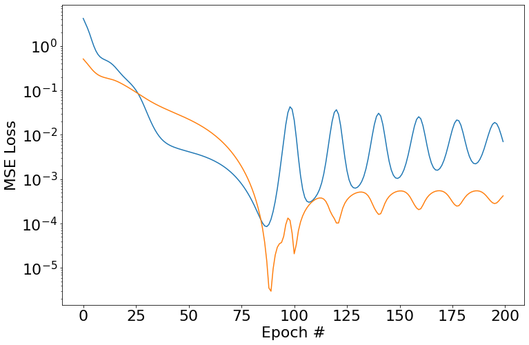
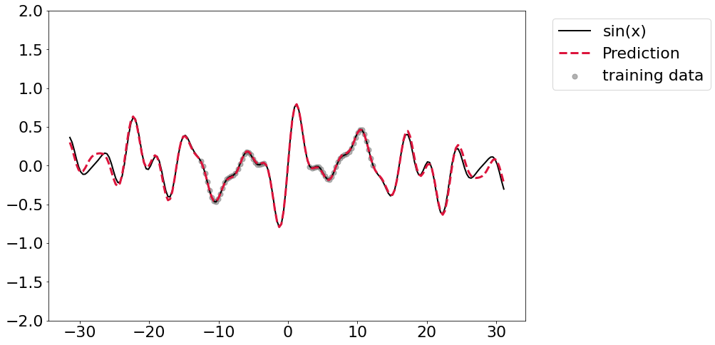
Adding regularization

It seems that adding regularization in the form of weight decay seems to offer generally better fits, but it’s still not perfectly converging.

width = 8
model = SineNet(width)
loss_fun = torch.nn.MSELoss()
opt = torch.optim.AdamW(model.parameters(), lr=0.001)

train_loss_history = []
valid_loss_history = []

max_epochs = 200
for i in tqdm(range(max_epochs)):
    train_loss, valid_loss = epoch(
        x_train,
        y_train,
        model,
        loss_fun,
        opt=opt,
        X_valid=x_valid,
        y_valid=y_valid
    )
    train_loss_history.append(train_loss)
    valid_loss_history.append(valid_loss)

plt.semilogy(train_loss_history)
plt.semilogy(valid_loss_history)
plt.xlabel('Epoch #')
plt.ylabel('MSE Loss')

png

y_pred = []
for x in x_truth:
    y_pred.append(model(torch.tensor([x/np.pi], dtype=dtype).flatten()).detach().numpy())

plt.plot(x_truth, y_truth, linewidth=2, color='black', label='sin(x)')
plt.scatter(x_train, y_train, color='grey', marker='.', alpha=0.6, s=200, label='training data')
plt.plot(x_truth, np.hstack(y_pred), linewidth=3, color='crimson', linestyle='--', label='Prediction')
plt.ylim([-2,2])
plt.legend(bbox_to_anchor=(1.04,1), loc="upper left")

png

Let’s overparameterize!

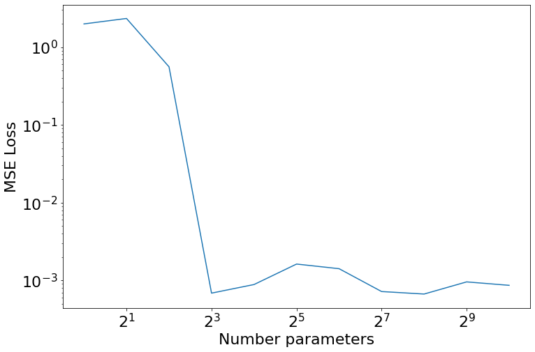
Of course, one of the main things we often do in machine learning is massively overparameterize the models. In some sense this is why we add regularization, but it’s also helpful in it’s own right. I was wondering if we’d be able to get some sort of double descent type behavior if we add more and more parameters to this problem. Here I’m just testing for “Model-wise double descent”, but expanding out to different max epochs to look for a signal there would be interesting (and related to the grokking paper

iterations_per_width = 20 # Repeat 20 trainings and take the one with the lowest training loss
widths_to_try = [1, 2, 4, 8, 16, 32, 64, 128, 256, 512, 1024]
max_epochs = 100

lowest_losses = []
best_models = []
for width in tqdm(widths_to_try):
    test_models = []
    test_losses = []

    # Sample 20 different trainings
    for i in range(iterations_per_width):
        model = SineNet(width)
        loss_fun = torch.nn.MSELoss()
        opt = torch.optim.AdamW(model.parameters(), lr=0.001)
        train_loss_history = []
        valid_loss_history = []
        for i in range(max_epochs):
            train_loss, valid_loss = epoch(
                x_train,
                y_train,
                model,
                loss_fun,
                opt=opt,
                X_valid=x_valid,
                y_valid=y_valid
            )
            train_loss_history.append(train_loss)
            valid_loss_history.append(valid_loss)
        test_models.append(model)
        test_losses.append(train_loss_history[-1])

    # Record the best loss and associated model
    lowest_loss_idx = np.argmin(test_losses)
    lowest_losses.append(test_losses[lowest_loss_idx])
    best_models.append(test_models[lowest_loss_idx])

plt.plot(widths_to_try, lowest_losses)
plt.gca().set_xscale('log', basex=2)
plt.gca().set_yscale('log', basey=10)
plt.xlabel('Number parameters')
plt.ylabel('MSE Loss')

png

Fin

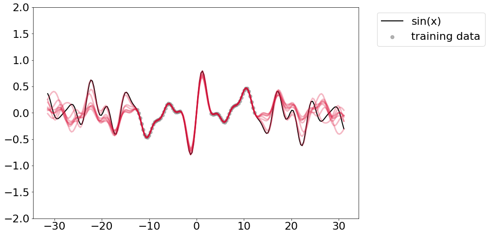
Okay, we see none of them ever made it to a perfect fit, but at 8 parameters we get a huge dropdown in loss, which is good since that’s hwo much model capacity we know we needed apriori. Anyhow, just some random messings around. I’ll leave you with the traces of all of those “best models”.

plt.plot(x_truth, y_truth, linewidth=2, color='black', label='sin(x)')
plt.scatter(x_train, y_train, color='grey', marker='.', alpha=0.6, s=200, label='training data')

for model in best_models[3:]:
    y_pred = []
    for x in x_truth:
        y_pred.append(model(torch.tensor([x/np.pi], dtype=dtype).flatten()).detach().numpy())
    plt.plot(x_truth, np.hstack(y_pred), linewidth=3, alpha=0.3, color='crimson', linestyle='-')
plt.ylim([-2,2])
plt.legend(bbox_to_anchor=(1.04,1), loc="upper left")

png