Sensitivity of the pseudoplastic basal sliding coefficient in CISM
Introduction
Motivation
Sea level rise due to ice sheet contributions remains a major source of uncertainty for Earth system models (Bromwich2010). This uncertainty stems from several factors, including incomplete process knowledge, inability to resolve heterogeneity in measurements, poor understanding of nonlinearities, and limits on computational capability (with the possible addition of other sources). Recent increases in the capabilities of remote sensing platforms have helped to build a clearer picture of these contributions. Glacial loss from ice sheets happens via two general mechanisms. First are surface mass balance (SMB) processes which include surface melt, meltwater runoff, sublimation, and losses due to wind; collectively these processes are referred to as ablation. The remainder of losses to the dynamical behavior of ice sheets, which includes processes such as surging, calving, and sliding.
Basal processes account for several of the most significant contributors to the dynamic behavior of ice sheets (Cuffey, 2010, Moon, 2012). In the last several decades two major loss events were shown to have contibutions from dynamical processes contributing more than 50% of the total loss (Kjaer, 2012).
Basal Slip
The terminology used to describe glacial motion at the ice/land interface has the tendency to be unclear. We adopt the terminology “basal slip” from Cuffey, 2010 to refer to all processes which involve motion due to both sliding and deformation at this interface. This relationship between the bottom of ice sheets and the subsurface has been associated with large uncertainty principally due to difficulty from observing this process, which also propogates forward into the ability to develop robust theory that is able to explain more easily measured quantities.
Generally, two categories have been developed from observations that have occurred. These motions will be referred to as hard and soft bed relationships. Hard bed glaciers are generally thought of as sliding over a non-deformable bedrock surface. Soft bed glaciers tend to have higher average velocities, and are associated with deformable sediment based medium in the subsurface. It is sometimes also useful to discuss a third type, which is a combination between glaciers and ice shelves floating above open water beyond the grounding line. Despite the emphasis placed on subsurface topography and geology, it is not generally the case that glaciers behave uniformly at a location in space, but rather exhibit a large amount of temporal variability as well, and can be seen in surging glaciers.
As a matter of notation we define the velocity at the bed as \(u_b\). Then, as a glacier flows at some rate there is an inverse reaction as described in Newton’s third law, which can be related to the shear stress which we will denote \(\tau_b\). Many formulations of this velocity-stress relationship have been explored to describe the dynamical motions of glaciers (see Cuffey, 2010 for an overview of methods). These relations are known as either slip or sliding relationships. We will refer to them as sliding relationships.
It has been shown that a pseudoplastic formulation of the sliding relationship is able to accurately reproduce the observed surface velocities of the Greenland ice sheet (Aschwanden, 2016). Plasticity of sliding relationships describes the ability for the glacial bed to deform. The form of the sliding relationship used is given as
\[\tau_b = tan(\phi) N \frac{u}{u_0^q |u|^{1-q}}\]where \(N \propto \rho g H\) is the effective pressure (which is reduced in presence of water), \(\phi\) is an elevation dependent friction angle, \(q\) is tunable exponent (1=linear, 0=plastic), and \(u_0\) is a threshold velocity.
Methods
This study was performed using a development branch of the Community Ice Sheet Model (CISM). The build of the code that was used is slated to be a minor point update release at the time of writing. The primary difference, for the sake of this analysis, is the addition of the pseudoplastic sliding law discussed previously. Model runs were conducted at a 4km resolution using the input datasets described in Joughin, 2010 and Bamber, 2013. The surface mass balance from the input dataset was augmented to set the surface mass balance of currently ice-free grid cells to -2mm/year. The reasons for this are twofold. First, the input dataset is untested, making certain calibrations and outputs hard to isolate. Second, it has been shown previously that this value provides a reasonable first order approximation to historical behaviors (Fyke, 2014).
Simulations were run diagnostically for 10kyr to reach steady state. Then, additional runs of 2kyr were run with finer temporal output to provide more representative aggregated values.
Runs were conducted at seven different values of \(q\), evenly spaced from \(q=0.3\) to \(q=0.6\). All other parameters were held constant for the durations of the runs. It should be noted up front (and will be reiterated) that runs for the \(q=0.35\) setup had convergence issues. Motivation for inclusion of their results will be provided.
Input data consisted of topographic information derived from a synthesis of remote sensing data products (Bamber 2013). The validation aspect of the dataset was also based on remote sensing data (Joughin, 2010). The majority of options and parameters were the same as those specified in the the InitMIP experiments.
Results
Distribution of mean quantities of interest
As was mentioned above, the extension runs for \(q=0.35\) had convergence issues, and did not run past the 24th output slice. All other values of \(q\) had 41 extension time slices, which will be examined. First, it was important to decide whether the \(q=0.35\) run was sufficiently stable to include in the following analyses. It should be noted that if future studies are performed this anomaly would be fixed before any analysis, but because of time constaints this was impractical.
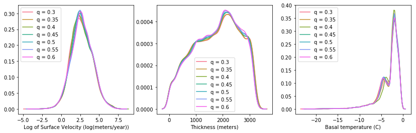
To determine whether the \(q=0.35\) extension run was valid we looked at the distributions of output variables for each of the runs was examined. From figure 1 we can see that the \(q=0.35\) distributions look like they’re within the spread of the other distributions. There are other interesting features in these distributions, but their discussion is omitted for the sake of brevity.
Sensitivity of velocity and thickness
The output data from the fine scale output was aggregated into data sets which were indexed on the different values of \(q\). Then, a linear regression was performed at each grid cell on thickness and surface velocity with respect to \(q\). Figures 2 and 3 show the results of these regressions.
Looking at these regressions we are interested in the areas where the slope is far from zero, and the \(r^2\) value is close to one. Areas where the \(r^2\) value is not close to 1 do not tell us anything about the effects of varying \(q\) on that particular measure.
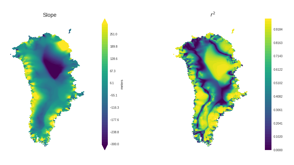
From figure 2 we can see that the northeastern interior sees a strong decrease in in the thickness as \(q\) increases. We also see a large increase in the thickness of the northeastern coastal region, which may be accounting for some of the losses inland. Other areas of interest tend to be along the coasts in the west and southeast. All of these locations show increases in thickness as \(q\) increases. We hypothesize that this is due to more flow from inland, where the thickness generally decreases slightly.
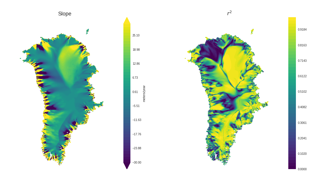
Figure 3 shows much more localized behaviors. Again, we see a strong effect on the northeastern section, with generally high values of \(r^2\) on the interior sections. This is a promising result, in that it may be possible to use \(q\) to tune for the ice stream which inhabits that region, and is generally poorly modeled. Again, the coasts along the western and southeastern region have particularly interesting to examine. Another feature of interest is the northwestern region, which has low \(r^2\) values over a large section, despite having very high signals in the regression. Investigation of this region temporally showed that this region was very dynamic within the model runs. For a better picture of the effect of \(q\) on this region either more time would be needed, or output would have to be written more often.
Comparison to observed surface velocities
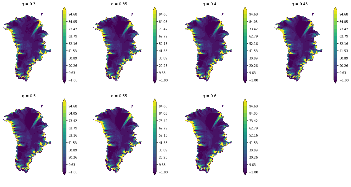
Figure 4 shows the difference in velocity for each of the runs conducted. Several key features stick out. First, the west coast, southeast coast, and northeastern ice stream are not well represented by any of the runs conducted. Second, we can see the high level of variability in the northwest corner as we did in the regressions. Generally, we also see higher values of \(q\) tend to capture the interior of the eastern and northern sections of the ice sheet marginally better than lower values. This observation is in line with Aschwanden, 2016.
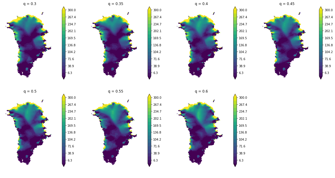
Figure 5 shows the differences in thickness. We see some general features that are common across all of the runs, namely the large underestimation of the thickness along the northern coast. It is unclear whether this is primarly a modeling or measurement error. We do see some differences among the values of \(q\) however. The decrease in thickness that can be seen in figure 5 ends up translating into an increase in error from the observations when \(q\) increases. The northern section of the west coast seems to get closer to observations as \(q\) increases.
Discussion
Sampling more parameter space
We have analyzed 7 runs varying a single parameter, leaving a large amount of the parameter space untested. Aschwanden, 2016 performed 15 experiments while varying 2 parameters (\(n\), and \(q\)). They found that the combination of \(q=0.6\) and \(n=3.25\) to provide the best fit with respect to surface velocity. To get a better understanding of the sensitivity of CISM’s pseudoplastic sliding law it would be useful to perform more runs that cover other parameter variations.
Low resolutions
Model runs were conducted at a 4km resolution, which may have limited fidelity of many outlet glaciers. It has been noted that Jakobshavn Isbræ, despite having an outlet width of roughly 10km, requires resolutions of 2km or less to accurately resolve the topography through which it flows. This dependence on resolution was found to be a large driver in the ability of simulations to reproduce observed flows (Aschwanden, 2016). We suspect that this is one of the major factors in the errrors seen along the west and southeastern coast for all of the parameter values.
A major factor in running higher resolution experiments is the increased cost due to computing. Taking into account a further exploration of the parameter space discussed previously could be used to develop hypotheses on parameter constraints. With smaller search spaces higher resolution simulations could be performed at less overall cost.
Conclusions
We found that several regions were particularly sensitive to the value of \(q\) when using a pseudoplastic sliding parameterization, but were unable to fully reproduce several key features in the surface velocity. Particularly difficult for the model to match were fine channels with high velocities, and the thickness in the northern regions. Analysis performed here was a very high level look at these effects.
Future work is planned to look at several things. To further explore the relationships between the observations a more quantitative look is being undertaken to look at certain regions specifically, as well as general error analysis for areas of high flow. There are several interesting areas of analysis of the basal temperature and melt that could provide insight into the transient behaviors of certain regions, such as the northwest that had very poor correlation coefficients for the velocity regression. Finally, we are also interested in the low frequency transient behavior of the basal states, which may not have been adequately removed from the datasets examined herein.
Acknowledgements
I would like to acknowledge the (very apprecated) help of Bill Lipscomb and Joseph Kennedy for their readiness to offer suggestions and logistical support throughout the course of this project. Ongoing work with them will hopefully result in further analysis along the lines discussed here as well as the development of a diagnostic tool that will be useful for future runs.
Additional thanks go out to Cecilia Bitz, the University of Washington Atmospheric Sciences Department, and National Center for Atmospheric Research for providing computing time and infrastructure that made this work possible.
References
Aschwanden, A., Fahnestock, M. A., and Truffer, M. (2016). Complex greenland outlet glacier flow captured. Nature Communications, 7:10524 EP –. Article.
Bamber, J. L., Griggs, J. A., Hurkmans, R. T. W. L., Dowdeswell, J. A., Gogineni, S. P., Howat, I., Mouginot, J., Paden, J., Palmer, S., Rignot, E., and Steinhage, D. (2013). A new bed elevation dataset for greenland. The Cryosphere, 7(2):499–510.
Bromwich, D. H. and Nicolas, J. P. (2010). Sea-level rise: Ice-sheet uncertainty. Nature Geosci, 3(9):596–597.
Cuffey, K. and Paterson, W. (2010). The physics of glaciers. Academic Press. glacier depth average velocity.
Fyke, J. G., Sacks, W. J., and Lipscomb, W. H. (2014). A technique for gener- ating consistent ice sheet initial conditions for coupled ice sheet/climate models. Geoscientific Model Development, 7(3):1183–1195.
Joughin, I., Smith, B. E., Howat, I. M., Scambos, T., and Moon, T. (2010). Greenland flow variability from ice-sheet-wide velocity mapping. Journal of Glaciol- ogy, 56(197):415–430.
Kjær, K. H., Khan, S. A., Korsgaard, N. J., Wahr, J., Bamber, J. L., Hurkmans, R., van den Broeke, M., Timm, L. H., Kjeldsen, K. K., Bjørk, A. A., Larsen, N. K., Jørgensen, L. T., Færch-Jensen, A., and Willerslev, E. (2012). Aerial photographs reveal late–20th-century dynamic ice loss in northwestern greenland. Science, 337(6094):569–573.
Moon, T., Joughin, I., Smith, B., and Howat, I. (2012). 21st-century evolution of greenland outlet glacier velocities. Science, 336(6081):576–578.